
Development of Electronic Structure Visualization Tools
It is a common practice to treat the chemical reactivity using a two-dimensional picture; charge-controlled reactions vs the orbital-controlled reactions. The partial atomic charges and molecular electrostatic potential (ESP) surface plots obtained from the calculated wavefunctions are extensively used to rationalize the charge-controlled processes. However, there are many systems where these computed quantities alone give an incomplete picture of reactivity. The common method to overcome the limitations of partial charges and ESP is to include the contributions of orbitals, and this is done by visualizing the frontier molecular orbitals. However, due to the delocalized nature of molecular orbitals, this method has a limitation of visualizing multiple pictures, not just one picture as used for ESP plots.
My Ph.D. work developed a descriptor of the electronic structure intended to more effectively bridge the gap between classical analyses of individual orbitals and the visualization of chemically intuitive quantities on the surface of the molecule. I developed the Electron Delocalization Range Function, \(EDR(\vec{r};d)\), and its derived interpretative tools, Orbital Overlap Distance, \(D(\vec{r})\), and Atomic-averaged Overlap Distance, \(D_A\). I applied these tools to study the electron delocalization in stretched and compressed chemical bonds, and as a partner to the electrostatic potential maps and atomic partial charges.
The major tool \(EDR(\vec{r};d)\) quantifies the extent to which the molecular orbitals around point \(\vec{r}\) in a calculated wavefunction overlap with a hydrogenic “test function” orbital of width \(d\) centered at \(\vec{r}\):
\[EDR(\vec{r} ; d)=\int d^3 \vec{r}^{\prime} g_d\left(\vec{r}, \vec{r}^{\prime}\right) \gamma\left(\vec{r}, \vec{r}^{\prime}\right),\]where the test function is given by
\[g_d\left(\vec{r}, \vec{r}^{\prime}\right)=\rho^{-\frac{1}{2}}(\vec{r})\left(\frac{2}{\pi d^2}\right)^{\frac{3}{4}} \exp \left(-\frac{\left|\vec{r}-\vec{r}^{\prime}\right|^2}{d^2}\right)\]Note that \(\gamma\left(\vec{r}, \vec{r}^{\prime}\right)=\sum_{i \sigma} n_{1 \sigma} \psi_{1 \sigma}(\vec{r}) \psi_{t \sigma}\left(\vec{r}^{\prime}\right)\) in Eq. 1 is the one-particle density matrix constructed from all of the spin-orbitals \(\psi_{t \sigma}(\vec{r})\) with nonzero occupancies \( n_{1 \sigma} \). In Eq. 2, the factor \(\left(\frac{2}{\pi d^2}\right)^{3 / 4}\) ensures that the value of the EDR is between -1 and +1. The Orbital Overlap Distance, \( D(\vec{r})\), is the value of \(d\) that maximizes \( EDR(\vec{r};d)\) at point \(\vec{r}\):
\[D(\vec{r})=\arg \max _d E D R(\vec{r} ; d).\]Atomic-averaged Overlap Distance, \(D_A\), is defined as the average value of orbital overlap distance in the points assigned to atom \( A\) in the molecule:
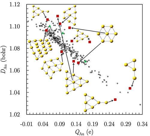
\[D_A=\int d^3 \vec{r} \rho(\vec{r}) D(\vec{r}) w_A(\vec{r}),\]where weight \( w_A(\vec{r})\) assigns point \(\vec{r}\) to atom \( \mathrm{A}\) in the molecule. I implemented these tools in an open-source wavefunction analysis package Multiwfn and Gaussian16 suite of programs. I also developed a stand-alone FORTRAN code for parallel evaluation of this toolkit. My implementations allow determining \(w_A(\vec{r})\) using Hirshfeld, Hirshfeld-I, Voroni, AIM, and Becke partitioning methods. Compact, chemically stable atoms tend to have \(D_A\) smaller than chemically soft, unstable atoms. Combining atomic charges and \(D_A\) captures trends in aromaticity, nucleophilicity, allotrope stability, and substituent effects. The chemical information provided by \(D_A\) becomes more significant in those cases where calculated charges alone do not provide the complete picture. For example, the carbon atoms of diamond, graphene, and \(\mathrm{C_{60}}\) have negligible and identical atomic charges but \(D_{\text{diamond}}=1.54\) bohr, \(D_{\text{graphene}}=1.58 \) bohr, \( D_{\mathrm{C_{60}}}=1.60 \) bohr, and \(D_{\mathrm{C_{\text{solaced}}}}=2.0 \) bohr illustrate the difference in their comparative reactivity and diamond’s thermodynamic stability. Figure below illustrates another example of \(D_A \)’s non-trivial predictions for metal clusters by capturing the site-dependent reactivity of \(\mathrm{Au_7{ }^{+}}\) hexagons. Partial charge alone provides limited insight into the most reactive parts of a cluster. Hexagonal \(\mathrm{Au_7{ }^{+}}\) has small \(D_{\text{Au}}\) in the outer ring and unusually large \(D_{\mathrm{Au}}\) for the central atom, although both atoms have nearly similar partial charges. Planar \(\mathrm{Au_9{ }^{+}}\) and \(\mathrm{Au_{10}{ }^{+}}\) show similar trends. This predicted reactivity of the central atom rationalizes a huge body of experimental data for facile doping of the central atom. Experiments confirm this structure for \( \mathrm{TiAu_6^{-}}, \mathrm{VAu_6^{-}}, \mathrm{CrAu_6^{-}}\), and \( \mathrm{YAu_6}\).
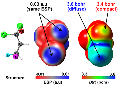
I applied \(D(\vec{r})\) plots to address the problems of medicinal chemistry, to distinguish the comparative reactivity of different carbon atoms at the defect sites of the graphene sheet, to quantify the reactivity of \(\mathrm{\sigma}\)-hole bonding (see illustration below) and to predict the values of Marcus \(\mu \)-scale of solvent softness. I used the mother tool \(EDR(\vec{r};d)\) to analyze the stretched and compressed chemical bonds and to show how this tool captures aspects of fractional occupancy, fractional charges, and left-right correlation in stretched covalent bonds.
For more details on these projects, refer to articles 3, 5, 7, 8, and 17 from my publications.